Finding the complete set of possible orderings

Another approach came from the observation, that often the actual number of possible orderings was small, although it could seem huge if only a small sub-set of the rows where considered. This is because some rows put severe restrictions on the positioning of other rows, thus limiting the number of orderings significantly. If all possible orderings of some sub-set could be generate at a moderate cost, all these orderings could be factorized, and we would be able to choose the minimal cost as the heuristic, thus producing a better (closer to lower-bound) heuristic.

This approach builds upon the idea of fixing one row position, but remembering what rows where candidates for that position. When fixing the next row, we hold the candidates together with the previous set of candidates, thus producing a set of possible orderings for these two rows. We continue this way, until we end up holding the set of possible orderings for the sub-system we where to calculate the heuristic for.

For the system

$$\left( \begin{array}{cccc} x & 0 & x & x \\ 0 & x & x & 0 \\ x & 0 & 0 & x \\ 0 & x & x & 0 \end{array} \right)$$

this can be illustrated as

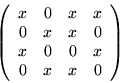
$$\begin{eqnarray*} &1:&\{ [r_1 \to p_1], [r_1 \to p_3], [r_1 \to p_4] \}\\ &2:&\... ... p_4, r_2 \to p_2], [r_1 \to p_4, r_2 \to p_3] \} \\ &3:&\ldots \end{eqnarray*}$$

where the mapping $[r_1 \to p_2]$ is interpreted as ``row one is fixed in position two''. The number to the left of the mappings represent the current ``depth'', eg. the number of rows we have fixed.

As is already seen in the mappings written before, the number of possible orderings easily explode. It is obviously a $\mathcal{NP}$ hard problem finding all orderings this way. Although the problem is complex, we may apply a little trick, to minimize the complexity. (The problem is still $\mathcal{NP}$ hard, but the actual run-time we see, will improve much with the little trick described below).

Remember that we order the columns ascending from left to right by the number of non-zeros they hold. Also, we should keep in mind that any valid ordering has strictly non-zeros in the diagonal. Thus, the top-most rows must have non-zeros to the left. Further on, we have the least number of choices for placing rows in the top, because the left-most columns hold the least number of non-zeros.

With the above observations, it should be clear, that if we start by fixing rows in the top locations, moving downwards, our algorithm will at all times consider the least number of possible orderings.

This approach produced a good heuristic on systems of sizes up to $n=40$. The run-time of a system of this size with density around $12\%$ was approximately 6 days on a standard PC. Much of the time was spent in actually calculating the cost of some ordering, because the number of orderings actually found was often large (in the order of $10^5$) and the run-time of the ordering itself was small compared to the number of orderings returned.

Limiting the number of orderings factorized to eg. 100, chosen randomly from the set of valid orderings, improved the run-time quite a lot (this was done in the 6 day run mentioned before). Still, the heuristic was good, even though it was only based on a hundred randomly chosen orderings out of several hundreds of thousands possible ones.

Still, the complexity of this approach killed it, when we where considering systems of the more realistic size above $n=40$. Even though the $\mathcal{NP}$ complexity was limited thru the trick described earlier, the algorithm still was $\mathcal{O}(n!)$ hard. On the system with $n=56$ and a density of approximately $12\%$ this algorithm did not complete in reasonable time (eg. the author's lack of patience preempted it after a week or so).

Still, based on numerous experiments with large more sparse systems, this algorithm behaves very well and produces good heuristics in reasonable time if only the sparsity can be kept well below $10\%$. It is absolutely a viable approach if the systems considered are very sparse.

<